The EY NextWave Data Science Challenge 2019 focuses on how data can help the next smart city thrive, and boost the mobility of the future.
As a challenge participant, I downloaded a dataset with a vast number of anonymous geolocation records from the US city of Atlanta (Georgia), during October 2018. my task is to produce a model that helps understand the journeys of citizens while they move in the city throughout the day. When digging deep into the challenge, I find the work could inspire solutions that help cities anticipate disruptions, make real-time decisions, design new services, and reshape infrastructures in order to become a city as smart as their citizens.
I have my team Wendy Huai, who is also from UCLA majoring stats.
Technically speaking, this is a predictive analysis that applied models to determine (binary classification) the response features based on other independent variables.
The evaluation standard is to check the accuracy score when applying the model (developed using training data) to the testing data and how well the model is built based on logic, run-time efficiency, generalization and space of tuning etc.
Here is an overview of the challenge:
- The variables in the dataset are as follows:
| Variable Name | Type | Description |
|---|---|---|
| hash | String | Represents the unique identifier of a device |
| trajectory_id | String | Represents the unique identifier of a trajectory associated to a device |
| time_entry* | Date | Indicates the local time for the starting point of the trajectory (HH:mm:ss) |
| time_exit* | Date | Indicates the local time for the ending point of the trajectory (HH:mm:ss) |
| Vmax | Integer | Represents the maximum velocity registered in the course of a trajectory. |
| Vmin | Integer | Represents the minimum velocity registered in the course of a trajectory. |
| Vmean | Integer | Represents the average velocity registered in the course of a trajectory. |
| x_entry | Double | Entry x coordinate (cartesian projected position) |
| y_entry | Double | Entry y coordinate (cartesian projected position) |
| x_exit | Double | Exit x coordinate (cartesian projected position) |
| y_exit | Double | Exit y coordinate (cartesian projected position) |
dimemsion: 67065 * 9
The challenge objective
I would like to predict how many people are in the city center between 15:00 and 16:00. The test dataset contains a number of devices where the trajectories after 15:00 have been removed. All but one: After 15:00, you will find one last trajectory, with (1) entry location, (2) entry time and an exit time that is between 15:00 and 16:00. But the exit point has been removed.
My task is to predict the location of this last exit point and whether this device is within the city center or not. The target variable is the latter.
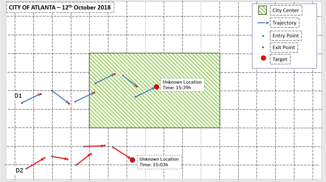
After I estimate the position of each target, I have to classify that point based on whether it is located inside the city center or not: See the graphic example below

The procedure
Overview – Exloration – Questioning – Data Inspection – Preprocessing (cleaning, imputation, manipulation, balancing, normalization, transformation …) – Stratified Data Spliting – Feature Engineering – Modeling – Tuning – Validation (CV,kV, LOOCV … ) – Testing – Evaluation (AUC/ROC, ConfusionMatrix …) – Re-tuning – Submission
There are 37 models I have built and featured using R and Python based on the running time and hands-on application during this competition, and they are (not limited to):
| Model Name | - | - |
|---|---|---|
| Logistirc Regression | Naive Bayesian | Regression Trees & Baggings |
| kNN | SVM | Random Forest |
| Gradient Boosting | Ensembled Model | LDA/QDA |
Sample submission
The submissions are csv files containing the information of trajectory_id with classfiation result 1/0 representing if the person is in city center or not.
Rankings
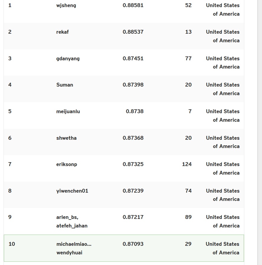
- Top 10 in US with quite less intense amount of submissions: 
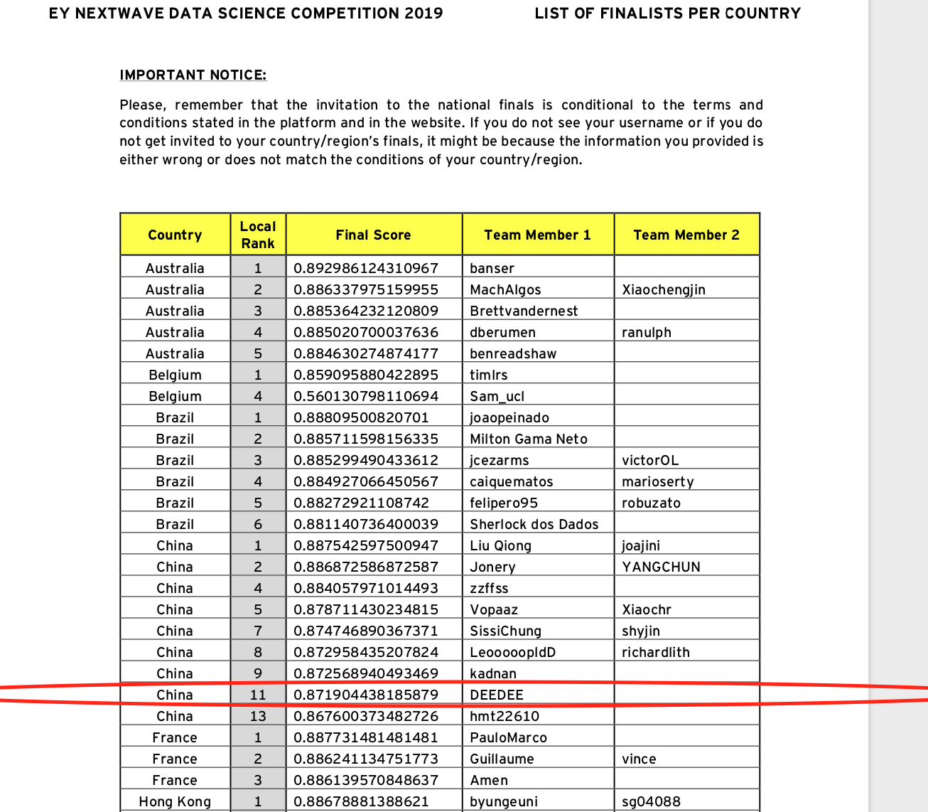
- Ranking 11 in China region under name DEEDEE as local finalist 
Improvement
 - we could improve the model with more advanced algorithms such as Generalized RF.
 - Imputate the missing values better
 - Balance the data distribution for some of the models
 - Create more variables given the 6* 67065 dimension, we can create more training features to optimize a best variable-observation ratio while still preventing from overfitting.
 - Conduct more cross validations.
Reference files:
Sample R code
 set.seed(16)
# n=use
new=n[sample(1:nrow(n),104268,replace = F),]
 # new=use
 train.index <- createDataPartition(new$target,p = .75, list = FALSE)
 new_train <- new[train.index,]
 new_test <- new[-train.index,]
set.seed(16)
ranger3 <- ranger(
    formula   = target ~ .,
    data      = new_train[,c(4,5,8,9,11,12,13,14,15,16,17)],
    num.trees = 500,
    mtry      = 8,
    sample.fraction = .55,
    min.node.size=5,
    importance = "impurity"
  )
rangepre3 <- predict(ranger3,new_test[,c(4,5,8,9,11,12,13,14,15,16,17)],type = "response")
pre3 <- ifelse(rangepre3$predictions>0.5,1,0)
errorrange3 <- mean(pre3!=new_test$target)
cat(1-errorrange3,"\n")

last <- read.csv("reallyuseuse.csv")
n=NULL
n=last
set.seed(71)

train.indexkk <- createDataPartition(new$target, p = .75, list = FALSE)
new_train <- new[train.indexkk, ]
new_test <- new[-train.indexkk, ]
features_train <- as.matrix(new_train[,c(3,4,5,6,22:33)])
response_train <- as.matrix(new_train[,9])
# names(new)
features_test <- as.matrix(new_test[,c(3,4,5,6,22:33)])
response_test <- as.matrix(new_test[,9])
# parameter list
params <- list(
  eta = .1,
    max_depth = 5,
    min_child_weight = 2,
    subsample = .8,
    colsample_bytree = .9
)
 set.seed(31)
# train final model
xgb.fit.final2 <- xgboost(
  params = params,
  data = features_train,
  label = response_train,
  nrounds = 410,
  objective = "reg:linear",
  verbose = 0
)
gbpre <- predict(xgb.fit.final2,features_test)
 gbpre <- ifelse(gbpre>0.5,1,0)
table(gbpre)
ggerror <- mean(gbpre!=response_test)
cat(1-ggerror)
Jiashu Miao June 18th 2019 :)